The Myth of the "Unrealizable" Filter
07 Mar 2012, 12:39 UTC
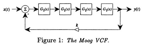
Sometimes you design a filter, and it contains a delay-free loop. This seems to happen most often when translating an analog circuit to discrete form (for instance, here the Moog VCF is analyzed, and this results in a discretization with a delay-free loop).
That paper throws its hands up and says, OK, let's introduce a delay, and then compensate using some pretty hairy maths and tables. This seems an odd solution since, as I will show below, the implementation of this filter is actually rather easy.
So, why are delay-free loops hard? Well, usually your filter output is a linear function of the filter state vector, S, and the current input x. S can contain functions of y(t-1), y(t-2), etc. so any delay-containing loop is encompassed. But a delay free loop means the output depends on y(t), which we do not yet know. This makes it impossible to directly translate the filter graph into code.
However, we can apply a little maths, and transform the filter into one which does not contain a delay-free loop.
Let us express a filter as follows:
y = F.S + fx
S' = G*S + xX
Here, F, X are vectors, G is a square matrix, and f is a scalar. x is the input sample and y is the output sample, while S is the filter state vector and S' is the updated filter state. These equations can be explained as follows:
yhas some amount of every state variable inSplus some amount ofx.- Each output state variable has some amount of every input state variable plus some amount of
x.
Now, let us add a delay-free loop. We replace x with h where h=x+ay. This puts a delay-free loop containing a scaler around the entire filter. So we have:
h = x + ay
y = F.S + fh
S' = G*S + hX
Now, a trivial amount of manipulation yields:
y = F.S + fx + fay
y = (F.S + fx)/(1-fa)
Then:
h = x + ay
S' = G*S + hX
Alternatively, you can insert the expression for y in terms of S and x into h, and then into G and X, giving back the original form of the state equations but with modified coefficients.
Note that the resulting filter is still linear, so this technique can be composed, and multiple loops can be placed in a hierarchical manner around combinations of such graphs. In fact, we can solve more generally for a delay-free network, which gives a set of simultaneous equations (in y, z, etc.). In this case, x and y are vectors, a is a |y|x|x| matrix, and f is an |x|x|y| matrix, so instead of a simple divide we end up needing invmat(I-fa), where (I-fa) is a |y|x|y| square matrix. (If this matrix is non-invertible, the filter really is unrealizable!)
Ultimately, if the filter is non-linear, then instead of a matrix inverse we need to find the inverse of a general non-linear function over a vector. The only effective way to do this, in many cases, is iteratively per sample i.e. using the recurrence for y inside a solver such as Successive Over Relaxation, or using a more complex technique such as Newton's Method.
An interesting point to note is that this technique implies that graphs can represent not only sequential programs, but constraints to be solved. By using delay-free loops to connect variables to themselves (or sets of variables to each other) we can represent any kind of equation, not only a closed-form expression (as in C++, for instance). The compilation of such graphs is a problem which may be solved simply in some cases (using the ideas above), may be solved in some cases using technologies such as Mathematica or Maple, but in the general case is not solvable without some iterative runtime solver (Spice does this). Fortunately, detection of each case is relatively simple - look for delay-free loops!
There is implied a connection between delay-free loops and closed-form expressions:
- If a graph contains no delay-free loops, it represents a closed-form expression, which can be directly evaluated.
- If a graph contains one or more delay-free loops, it represents a system which must be solved. This solution may be achievable offline, transforming the graph into a closed-form graph, or it may only be approximable at runtime.
Thanks to Dave Christensen for pointing out a typo which suggested some improvements to the whole article!